
In the last module, we predicted how much (numbers). In this module, we are learning how to predict which one (categories).
If Regression is about drawing a line through points, Classification is about drawing a line that separates groups.

4.1 What is Classification? (The Sorting Hat)
Classification is the process of taking an input and putting it into a specific “bucket” or category.
Binary vs. Multi-class
- Binary Classification: Only two buckets. (e.g., Is this email Spam or Not Spam? Is this transaction Fraud or Legit?)
- Multi-class Classification: More than two buckets. (e.g., Is this a photo of a Dog, Cat, or Bird? Is this iris flower a Setosa, Versicolor, or Virginica?)
4.2 Logistic Regression: The Name is a Trick
Here is a secret that confuses every beginner: Logistic Regression is used for Classification, not Regression.
How it works: The Sigmoid Curve
While Linear Regression draws a straight line that goes on forever, Logistic Regression uses a special curve called the Sigmoid Function.
- It takes any number and “squashes” it to be between 0 and 1.
- This result is treated as a Probability. If the model outputs 0.85, it’s saying “I’m 85% sure this is Spam.”
The Decision Boundary
Once we have that percentage, we set a “line in the sand” (usually at 0.5).
- Above 0.5? It’s Category A.
- Below 0.5? It’s Category B.
4.3 Implementing Classification in Python
Let’s look at a practical example: building a “Spam Filter” for your inbox. code Pythondownloadcontent_copyexpand_less
from sklearn.model_selection import train_test_split
from sklearn.linear_model import LogisticRegression

# 1. Imagine our data: X (Email Length, Number of Typos), y (1 for Spam, 0 for Not Spam)
X = [[100, 5], [10, 0], [500, 20], [15, 1]] # Examples
y = [1, 0, 1, 0] # Labels

# 2. Split into Training and Testing sets
X_train, X_test, y_train, y_test = train_test_split(X, y, test_size=0.25)

# 3. Create the "Classifier"
classifier = LogisticRegression()

# 4. Train the model
classifier.fit(X_train, y_train)

# 5. Make a prediction for a new email
# (e.g., 200 words long with 10 typos)
new_email = [[200, 10]]
prediction = classifier.predict(new_email)

print(f"Prediction (1=Spam, 0=Not Spam): {prediction[0]}")
4.4 Evaluating the Model: Why Accuracy is Often a Liar
In Regression, we used MSE. In Classification, we use a Confusion Matrix.
The Problem with Accuracy
Imagine you have a test for a very rare disease that only 1 in 1,000 people have. If I build a “model” that just guesses “No Disease” for everyone, I will be 99.9% accurate. But I’m a terrible doctor because I missed the person who actually needed help!
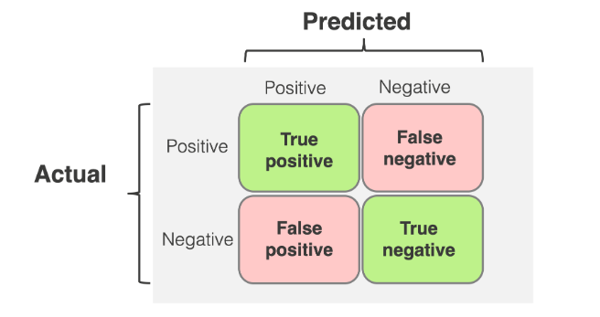
The Confusion Matrix: 4 Important Boxes
- True Positive (TP): You said “Spam,” and it was Spam. (Good!)
- True Negative (TN): You said “Safe,” and it was Safe. (Good!)
- False Positive (FP): You said “Spam,” but it was a message from your Grandma! (The “False Alarm”)
- False Negative (FN): You said “Safe,” but it was a virus. (The “Missed Danger”)
Key Metrics to Remember:
- Precision: “When I guess Spam, how often am I right?”
- Recall: “Of all the actual Spam emails, how many did I catch?”
- F1-Score: The perfect balance between Precision and Recall.
4.5 Decision Trees: The “Flowchart” Method
If Logistic Regression is about math and probabilities, a Decision Tree is about logic. It’s like playing a game of “20 Questions.”
- Step 1: Is the email longer than 100 words? (Yes/No)
- Step 2: Does it contain the word “Free”? (Yes/No)
- Step 3: Is the sender in your contacts? (Yes/No)
Why use them? They are incredibly interpretable. You can literally print out the tree and see why the computer made its decision. This makes them a favorite for business meetings where you need to explain the “logic” behind the AI.
Module 4 Summary
You’ve now mastered the two pillars of Supervised Learning: Regression (Numbers) and Classification (Categories). You know that Logistic Regression is actually a classifier, you know how to read a Confusion Matrix, and you’ve seen how Decision Trees use logic to reach a conclusion.
In our next and final module, we’ll see what happens when the computer has to learn without any labels!