
Now that we have clean, polished data, it’s time for the “magic” to happen. This is the module where you stop being a data cleaner and start becoming a Machine Learning builder.
We are starting with Regression, which is the bread and butter of the prediction world.
3.1 What is Supervised Learning? (The Teacher-Student Model)
Imagine you are teaching a child to recognize the relationship between the size of a toy and its price. You show them 10 toys, tell them the size of each, and tell them exactly how much each costs.
This is Supervised Learning.
- The “Supervision”: You are providing the “Answers” (Labels) to the computer.
- The Goal: The computer learns the pattern so that when you show it a new toy it has never seen before, it can guess the price accurately.
What is a “Regression” Task?
In ML, we use Regression whenever the answer we want to predict is a continuous number.
- Will it rain tomorrow? (That’s NOT regression; that’s a Yes/No).
- How many inches of rain will fall tomorrow? (That IS regression).
Real-World Examples:
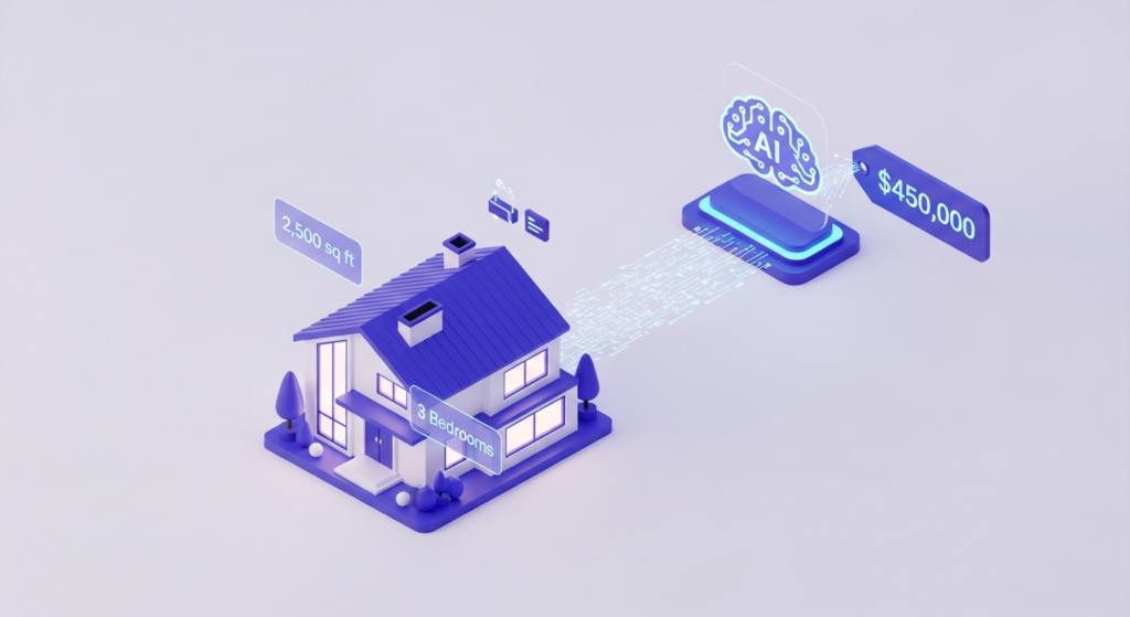
- Predicting the price of a house based on square footage.
- Estimating how many units of a product will sell next month.
- Predicting the temperature for next Tuesday.
3.2 Linear Regression Intuition: Finding the “Best Fit”
Linear Regression is the simplest and most famous algorithm in the world. Its goal is to draw a straight line through your data points.
The “Line of Best Fit”
Imagine a scatter plot of house sizes (horizontal axis) and prices (vertical axis). Generally, as size goes up, price goes up. Linear Regression tries to draw a single straight line that passes as close as possible to all those dots.
- The Slope: How much does the price increase for every extra square foot?
- The Intercept: If a house had zero square feet (theoretically), what would the price be?
Minimizing the “Ouch” (Errors)
How does the computer know where to draw the line? It looks at the “distance” between the actual data points and the line it drew. These distances are Errors.
The most common way to measure this is Mean Squared Error (MSE). The computer keeps “wiggling” the line until those errors are as small as humanly possible.
3.3 Implementing Linear Regression in Python
Thanks to a library called Scikit-Learn (sklearn), you don’t have to do the heavy math yourself. The workflow usually follows these four steps:
- Split: We divide our data into a Training Set (to learn from) and a Test Set (to test the model’s memory).
- Initialize: We tell Python we want to use the LinearRegression “tool.”
- Fit: This is the actual “Learning” phase. We give the model the training data.
- Predict: We ask the model to guess the prices for the test data.
The Code Look-alike:
from sklearn.model_selection import train_test_split
from sklearn.linear_model import LinearRegression

# 1. Split the data (80% training, 20% testing)
X_train, X_test, y_train, y_test = train_test_split(X, y, test_size=0.2)

# 2. Create the model
model = LinearRegression()

# 3. Train the model (The "Learning" part)
model.fit(X_train, y_train)

# 4. Make predictions
predictions = model.predict(X_test)
To make this concrete, let’s imagine we are working for a real estate agency. We want to predict a House Price based on its Square Footage. Here is how that looks in actual Python code.
The Practical Example: Predicting House Prices
import numpy as np
import pandas as pd
from sklearn.model_selection import train_test_split
from sklearn.linear_model import LinearRegression

# 1. Imagine our data: X (Square Feet) and y (Price in $)
# Usually, you'd load this from a CSV file
data = {
    'sq_feet': [1500, 1800, 2400, 3000, 3500, 4000],
    'price': [300000, 350000, 450000, 550000, 620000, 710000]
}
df = pd.DataFrame(data)

# Features (X) must be a 2D array, Labels (y) is 1D
X = df[['sq_feet']]
y = df['price']

# 2. Split: 80% to learn, 20% for the "Final Exam"
X_train, X_test, y_train, y_test = train_test_split(X, y, test_size=0.2, random_state=42)

# 3. Initialize the Model
model = LinearRegression()

# 4. Train: The model finds the "Best Fit Line"
model.fit(X_train, y_train)

# 5. Predict: Let's guess the price for a 2800 sq ft house
new_house = np.array([[2800]])
predicted_price = model.predict(new_house)

print(f"A 2800 sq ft house is predicted to cost: ${predicted_price[0]:,.2f}")
3.4 Evaluating the Model: How Good are We?
After the model makes its guesses, we need to “grade” it. We compare its predictions to the actual answers (the labels).
The Three Main Metrics:
- Mean Absolute Error (MAE): On average, how many dollars was the model off by? (Very easy to explain to a boss).
- Mean Squared Error (MSE): Similar to MAE, but it “punishes” big mistakes more severely.
- R-Squared (
R2R^2R2): This is a score between 0 and 1 (or 0% to 100%). It tells you how much of the variation in the data your model actually explains.- 0.90: Your model is a genius.
- 0.20: Your model is basically just guessing.
🛠 Hands-on Lab: Predicting Sales
Let’s imagine you are a marketing manager. You have a dataset of how much money was spent on TV ads and the resulting sales.
Your Goal: Build a model that predicts sales based on ad spend.
- Load the data using Pandas.
- Split the data into features (TV Spend) and labels (Sales).
- Train your Linear Regression model.
- Evaluate: Calculate the R-squared value. If it’s high, congratulations! You can now tell your boss exactly how much sales to expect if you increase the TV budget.
Module 3 Summary
You’ve just moved from “Data Analyst” to “Machine Learning Engineer.” You understand that Supervised Learning needs labels, Regression is for predicting numbers, and Linear Regression is all about finding that perfect “best fit” line.
Next up: Classification—where we teach the computer how to put things into categories!