
Logistic regression. The name might sound complex, but at its heart, it’s a remarkably intuitive and incredibly useful algorithm. Think of it as your reliable workhorse for tackling problems where you need to predict categories rather than continuous numbers. It’s about answering the “yes” or “no,” the “this” or “that,” the “spam” or “not spam” question.
Instead of predicting a value on a sliding scale, logistic regression estimates the probability of something belonging to a specific group. It achieves this by transforming a linear equation’s output using a clever mathematical function called the sigmoid. This sigmoid function squashes the result into a neat range between 0 and 1, directly representing the likelihood of belonging to the positive class – your “yes,” your “spam,” your target category.
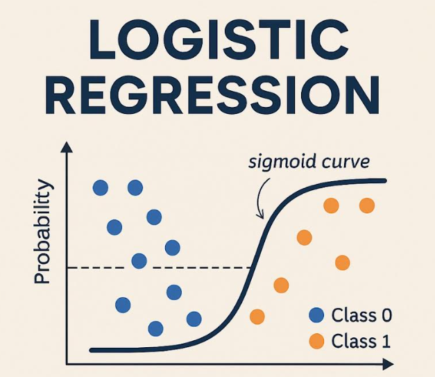
At its core, logistic regression estimates the probability that a given input belongs to a particular category—typically 0 or 1. It does this by applying the sigmoid function to a linear combination of input features:
Sigma(z) = 1 / (1 + exp(-z)), where z = w^T * x + b
- Sigma(z) or Sigmoid(z): The name of the function.
- exp(-z): e raised to the power of -z.
- w^T: w transpose (representing the weight vector).
- x: The feature vector.
- b: The bias term.
Why Choose Logistic Regression for Your Project?
Why reach for logistic regression when you have a whole toolbox of machine learning algorithms? Here’s the compelling case:
- Clarity of Insight: The model’s coefficients aren’t just numbers; they provide valuable hints about how different features influence the probability of the outcome you’re trying to predict.
- Speed and Efficiency: Logistic regression is a lean, mean computing machine. It can handle large datasets without bogging down your system.
- Quantifiable Confidence: It spits out probabilities, not just flat predictions. This allows you to understand how confident the model is in each prediction.
- Wide Applicability: From predicting customer behavior to diagnosing medical conditions, logistic regression shines in diverse fields.
Real-World Applications You Might Not Have Realized
Logistic regression is a silent powerhouse behind many applications you encounter daily:
- Healthcare: Assessing the risk of a patient developing a specific illness based on their medical data.
- Finance: Determining the creditworthiness of loan applicants to minimize risk.
- Email Filtering: Identifying and filtering out spam messages from your inbox.
- Marketing Analytics: Predicting which customers are most likely to churn or identifying promising leads for sales teams.
This squashes the output into a range between 0 and 1, making it ideal for probability-based classification.
Let’s Code: Building Your First Logistic Regression Model in Python
Now for the fun part! Let’s build a logistic regression model from scratch using Python’s scikit-learn library. We’ll start with a synthetic dataset for demonstration purposes.
Dissecting the Code below
- Synthetic Data Creation: We conjure a dataset with two features (X) and a binary target variable (y). Replace this with your data loaded from a CSV, database, etc. The random_state ensures the dataset generated is always the same.
- Data Partitioning: The train_test_split function carves the data into training and testing sets. The model learns from the training data, and then we test its mettle on the unseen testing data.
- Model Instantiation and Training: We bring a LogisticRegression model to life and train it using the fit method. The solver parameter dictates the optimization algorithm; ‘liblinear’ works well for smaller datasets.
- Prediction Time: We unleash the trained model to predict the class labels for the test set.
- Performance Evaluation: We measure the model’s success using accuracy, the confusion matrix, and a classification report.
- Accuracy: The percentage of correct classifications.
- Confusion Matrix: Reveals true positives, true negatives, false positives, and false negatives.
- Classification Report: Gives you precision, recall, F1-score, and support.
- Visualization: Plotting the confusion matrix and decision boundary to help understand the model’s performance.
Code (Python):
import numpy as np
from sklearn.model_selection import train_test_split
from sklearn.linear_model import LogisticRegression
from sklearn.metrics import accuracy_score, confusion_matrix, classification_report
import matplotlib.pyplot as plt
import seaborn as sns  # for heatmap

# 1. Create a Synthetic Dataset (replace with your own real-world data)
np.random.seed(0)  # Ensure consistent results
X = np.random.rand(100, 2)  # 100 data points, each with 2 features
y = (X[:, 0] + X[:, 1] > 1).astype(int)  # Binary target: 1 if sum of features > 1, else 0

# 2. Divide the Data into Training and Testing Subsets
X_train, X_test, y_train, y_test = train_test_split(X, y, test_size=0.2, random_state=42)

# 3. Instantiate and Train the Logistic Regression Model
model = LogisticRegression(solver='liblinear', random_state=42)  # 'liblinear' is suitable for smaller datasets
model.fit(X_train, y_train)

# 4. Generate Predictions on the Test Data
y_pred = model.predict(X_test)

# 5. Evaluate the Model's Performance
accuracy = accuracy_score(y_test, y_pred)
print(f"Accuracy: {accuracy}")

conf_matrix = confusion_matrix(y_test, y_pred)
print("Confusion Matrix:\n", conf_matrix)

class_report = classification_report(y_test, y_pred)
print("Classification Report:\n", class_report)

# Visualize the confusion matrix
plt.figure(figsize=(8, 6))
sns.heatmap(conf_matrix, annot=True, fmt='d', cmap='Blues',
            xticklabels=['Predicted 0', 'Predicted 1'],
            yticklabels=['Actual 0', 'Actual 1'])
plt.title('Confusion Matrix')
plt.ylabel('Actual')
plt.xlabel('Predicted')
plt.show()

# Visualize the Decision Boundary (only works well for 2 features)
plt.figure(figsize=(8, 6))
plt.scatter(X_test[:, 0], X_test[:, 1], c=y_test, cmap='viridis', label='Actual')

# Create a meshgrid to plot the decision boundary
xx, yy = np.meshgrid(np.linspace(X[:, 0].min() - 0.1, X[:, 0].max() + 0.1, 100),
                     np.linspace(X[:, 1].min() - 0.1, X[:, 1].max() + 0.1, 100))
Z = model.predict(np.c_[xx.ravel(), yy.ravel()])
Z = Z.reshape(xx.shape)

# Plot the decision boundary
plt.contourf(xx, yy, Z, alpha=0.4, cmap='viridis')
plt.xlabel('Feature 1')
plt.ylabel('Feature 2')
plt.title('Logistic Regression Decision Boundary')
plt.legend()
plt.show()
Critical Considerations
- Data Preprocessing is Key: Logistic regression thrives on well-prepared data. Consider scaling your features (using StandardScaler or MinMaxScaler) to boost performance. Feature scaling is important to ensure features with larger values don’t disproportionately influence the model.
- Feature Engineering: Craft your features carefully to provide the model with the most informative signals.
- Regularization: Guard against overfitting (where the model memorizes the training data but performs poorly on new data) with regularization techniques like L1 or L2. Adjust the C parameter to control regularization strength (smaller C = stronger regularization).
- Handling Multiple Classes: Logistic regression can be adapted for multi-class problems using techniques like One-vs-Rest (OvR) or Multinomial Logistic Regression.
- Addressing Class Imbalance: If one class significantly outnumbers the others, use techniques like oversampling or undersampling to create a more balanced dataset.
Final Thoughts
Logistic regression is a fundamental and powerful classification algorithm. By grasping its principles and putting it into practice with Python, you’ll gain a valuable tool for solving a wide range of real-world problems. Don’t hesitate to experiment and refine your approach to unlock its full potential!