
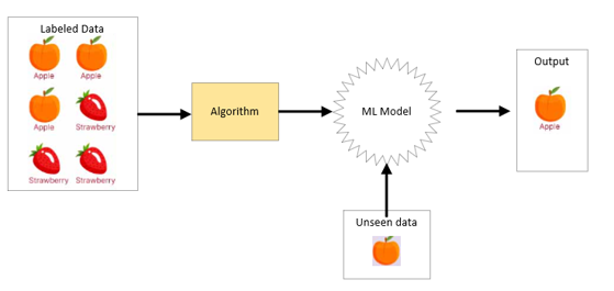
Imagine guiding a young child to recognize different fruits. You show them an apple and say “apple,” then a banana and say “banana,” and so forth. Eventually, the child learns to distinguish these fruits independently because they’ve been given labeled examples. This core concept underlies supervised learning in artificial intelligence.
Supervised learning is a type of machine learning where an algorithm learns a relationship between input data and output data by studying labeled examples. Think of it as learning under instruction – a “teacher” provides the correct answers (labels) for the input data, and the algorithm strives to grasp the underlying connection. Once trained, this algorithm can then forecast the output for new, previously unseen input data.
This potent technique fuels numerous applications, from filtering unwanted emails in your inbox to aiding in medical diagnoses and powering autonomous vehicles. However, before we delve deeper, let’s explore the diverse forms of supervised learning:
1. Classification: Organizing into Categories
Classification is akin to sorting items into distinct groups based on their attributes. In supervised learning, the objective of a classification algorithm is to assign data points to predefined groups or classes. The output variable in classification is categorical, meaning it belongs to a limited set of distinct values.
Example:
- Input Data: Electronic messages characterized by features like sender’s address, subject line content, and message body.
- Labels: “Junk” or “Not Junk.”
- Goal: Develop an algorithm capable of categorizing new incoming messages as either junk or not junk by recognizing patterns learned from the labeled examples.
Exploring Common Classification Algorithms:
Logistic Regression:
- Despite its name suggesting regression, this is a widely used algorithm for binary classification tasks (outcomes with two possibilities, such as “yes/no” or “true/false”).
- It models the likelihood of an outcome belonging to a specific category using a sigmoid function (also known as the logistic function). This function transforms a linear combination of input features into a probability between 0 and 1.
- It learns feature weights to best differentiate the two classes, establishing a decision boundary (typically at a probability of 0.5) for classifying new data. It’s straightforward, computationally efficient, and provides probability estimations, but can struggle with complex, non-linear data and is susceptible to outliers. It’s often used for predicting binary outcomes like customer churn or disease presence.
Support Vector Machines (SVMs):
- SVM aims to identify the optimal dividing line (hyperplane) that best separates different classes within the data’s feature space.
- The “support vectors,” which are the data points closest to this hyperplane, are crucial in defining it. The goal is to maximize the margin, which is the distance between the hyperplane and the nearest data points of each class. For data that isn’t easily separated by a straight line, SVM employs the kernel trick. Kernel functions map the data into a higher-dimensional space where a linear hyperplane can effectively separate the classes without explicitly performing complex calculations. Common kernel types include linear, polynomial, and radial basis function (RBF).
- SVMs excel in high-dimensional spaces and are robust against overfitting, especially with proper adjustments. They are versatile due to kernel functions, enabling them to handle non-linear data. However, they can be computationally demanding for large datasets, and selecting the right kernel and its settings requires careful tuning. They are often used in image and text classification.
Decision Trees and Random Forests:
- Decision Trees: A decision tree is a structure resembling a flowchart where each internal node tests a specific feature, each branch represents the outcome of that test, and each leaf node indicates a class label.
- The algorithm recursively divides the data based on the feature that best distinguishes the classes until a stopping point is reached. The splitting process aims to maximize information gain or minimize impurity using metrics like Gini impurity or entropy. To classify a new instance, you follow the path from the root node down to a leaf node based on the instance’s feature values.
- Decision trees are easy to understand and can handle various data types and non-linear relationships, and feature importance is readily determined. However, they are prone to overfitting and can be sensitive to minor data changes.
- Random Forests: A random forest is an ensemble learning method that combines numerous individual decision trees. Each tree in the forest is trained on a random sample of the data (with replacement, known as bootstrapping) and a random subset of the features. For classification, the final prediction is determined by the majority vote among the predictions of all the trees.
- This randomness helps reduce overfitting and improves the model’s ability to generalize to new data. While generally more accurate and robust than individual decision trees and capable of handling high-dimensional data, random forests are less interpretable and can be computationally intensive to train. They are widely used in areas like risk assessment and fraud detection.
Naive Bayes:
- This is a probabilistic classifier grounded in Bayes’ theorem. The “naive” aspect comes from its simplifying assumption that all features are independent of each other given the class label.
- Despite this often unrealistic assumption, Naive Bayes can perform surprisingly well, particularly in text-related classification tasks. It calculates the probability of a data point belonging to a specific class based on the prior probabilities of the classes and the likelihood of the features given the class. Bayes’ theorem provides a framework for updating the initial belief (prior probability) about a class based on new evidence (the features).
- Naive Bayes is simple, fast to train, effective with high-dimensional data, and requires relatively little training data. However, the naive independence assumption can be a significant limitation, and it can encounter issues if a feature value doesn’t appear with a particular class in the training data. It’s commonly used for spam filtering and sentiment analysis.
K-Nearest Neighbors (KNN):
- KNN is a non-parametric, instance-based learning algorithm. It doesn’t build an explicit model during training. Instead, to classify a new data point, it identifies the k closest data points in the training data based on a distance measure (e.g., Euclidean distance).
- The class of the new data point is then determined by the most frequent class among these k neighbors. The choice of k is critical; a small k can make the model susceptible to noise, while a large k can smooth decision boundaries but might include irrelevant points. KNN is easy to grasp and implement, handles multi-class problems well, and can capture complex decision boundaries. However, it can be computationally expensive for large datasets during prediction, is sensitive to the choice of k and the distance metric, and feature scaling is important. It also doesn’t perform well in high-dimensional spaces due to the “curse of dimensionality.” It finds applications in recommender systems and pattern recognition.
2. Regression: Predicting Continuous Values
In contrast to classification, where the output is a category, regression focuses on predicting continuous numerical values. Think of it as trying to forecast a quantity based on related factors.
Example:
- Input Data: Characteristics of houses such as size in square feet, number of bedrooms, number of bathrooms, and location.
- Labels: The corresponding sale price of each house.
- Goal: Train an algorithm to estimate the sale price of a new house based on its features.
Exploring Common Regression Algorithms:
Linear Regression:
At its heart, linear regression tries to find the best-fitting straight line that describes the relationship between a dependent variable (the thing you’re trying to predict or explain) and one or more independent variables (the things you think might be influencing it).
- Dependent Variable (Y): This is the outcome you’re interested in. It’s often called the response variable or the target variable. Think of it as what you’re trying to predict.
- Independent Variable (X): This is the factor you believe might influence the dependent variable. It’s also known as the predictor variable or the feature. You’re using this to make your prediction.
Imagine This: Let’s say you’re a plant enthusiast, and you suspect that the amount of sunlight a plant receives affects its growth.
- Dependent Variable (Y): Plant height (what you want to predict).
- Independent Variable (X): Hours of sunlight per day.
Linear regression will try to find a line that best describes how plant height changes as the amount of sunlight increases or decreases.
The Equation of the Line: The line that linear regression finds can be represented by a simple equation:
Y = a + bX
Where:
- Y is the predicted value of the dependent variable.
- X is the value of the independent variable.
- a is the y-intercept (the value of Y when X is 0). In our plant example, this might represent the initial height of the plant before it gets any sunlight, though that might not be a meaningful real-world value.
- b is the slope of the line (how much Y changes for every one-unit change in X). This is the key: it tells you how much the plant height is expected to increase for each additional hour of sunlight.
Simple vs. Multiple Linear Regression
- Simple Linear Regression: Uses one independent variable to predict the dependent variable (like our plant example).
- Multiple Linear Regression: Uses multiple independent variables to predict the dependent variable. For example, plant height might be affected by sunlight and the amount of water it receives and the type of soil it’s planted in. The equation becomes more complex, but the core idea is the same: find the best-fitting relationship.
How Does It Work?
Linear regression uses a method (often called “least squares”) to find the line that minimizes the distance between the actual data points and the predicted values on the line. Think of it as trying to draw a line through a scatter plot of data points, so the line is as close as possible to all the points.
Support Vector Regression (SVR):
- SVR extends the principles of Support Vector Machines (SVM) to regression problems. Instead of finding a hyperplane that separates classes, SVR aims to find a function that comes within a certain tolerance ((\epsilon)) of all the data points. The objective is to minimize errors outside this margin while keeping the function as simple as possible to promote generalization. Similar to SVM, SVR utilizes kernel functions to handle non-linear relationships. The (\epsilon)-insensitive loss function is often used, meaning errors within the (\epsilon) margin are not penalized. Only data points outside this margin (the support vectors) influence the model. SVR is effective in high-dimensional spaces, robust to outliers due to the (\epsilon) margin, and can model non-linear data using kernels. However, it can be computationally intensive for large datasets, and selecting appropriate kernel parameters (including (\epsilon)) requires careful tuning. It’s often used for forecasting financial data or predicting system performance.
Decision Tree Regression and Random Forest Regression:
- Decision Tree Regression: Similar to decision tree classification, but instead of predicting a class at the leaf nodes, it predicts a continuous value (typically the average or median of the target variable for the data points in that leaf). The splitting criteria also differ, aiming to minimize the variance or mean squared error within the resulting segments.
- Random Forest Regression: This is an ensemble method comprising multiple decision tree regressors. Each tree is trained on a random subset of the data and a random subset of the features. The final prediction is the average (or median) of the predictions from all the individual trees. Both types can model non-linear relationships and handle mixed data types. Single decision trees are easy to interpret, while random forests are generally more accurate and less prone to overfitting. However, single decision trees can overfit and be unstable, and random forests are less interpretable and can be computationally expensive. They are used in various prediction tasks, such as estimating property values or predicting product demand.
The Supervised Learning Process:
The general steps involved in supervised learning typically include:
- Data Gathering and Preparation: Collecting labeled data and preparing it by cleaning, transforming, and dividing it into training and testing sets.
- Algorithm Selection: Choosing an appropriate supervised learning algorithm based on the problem type and data characteristics.
- Model Training: Feeding the training data to the selected algorithm to learn the relationship between inputs and outputs.
- Model Evaluation: Assessing the trained model’s performance on the unseen testing data using relevant metrics (e.g., accuracy for classification, mean squared error for regression).
- Model Deployment: Using the trained model to make predictions on new, real-world data.
In Conclusion:
Supervised learning is a cornerstone of machine learning, offering powerful tools for prediction and categorization. By understanding the different types of supervised learning – classification and regression – and the array of algorithms available, you can begin to tackle a wide spectrum of real-world challenges. As you advance in your machine learning journey, remember that experimentation and a deep understanding of each algorithm’s strengths and limitations are crucial for building effective and reliable predictive models.