Module 1: The ML Workflow & Data Basics

Welcome! In this first module, we are going to demystify Machine Learning (ML). Forget the sci-fi movies for a second; at its core, ML is just a way to teach a computer to find patterns in data so it can make smart guesses about the future.

By the end of this module, you’ll understand the “lifecycle” of an ML project, how to talk about data like a pro, and how to use Python to peek inside a dataset.

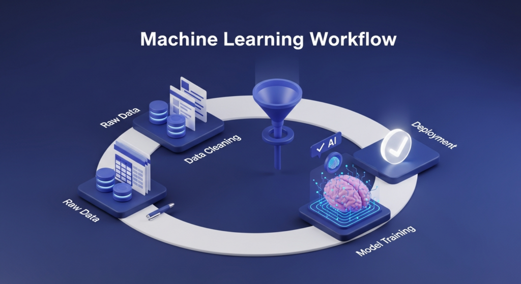
1.1 The Machine Learning Workflow: The “Cooking” Analogy

Think of building an ML model like opening a restaurant. You don’t just walk into a kitchen and start cooking. There’s a process.

The 6-Step Cycle

Problem Definition (The Menu):
You have to decide what you’re making. In ML, we ask: “What are we predicting?”
- Example: Are we predicting if a credit card transaction is “Fraud” or “Legit”? If you don’t define this clearly, you’ll build a model that solves the wrong problem.
Data Collection (Sourcing Ingredients):
You need raw material. This could be sensors, customer logs, or public datasets.
- Pro Tip: The quality of your model depends entirely on the quality of your data. If you use rotten ingredients, the meal will be terrible.
Data Preprocessing (Prepping the Veggies):
Raw data is messy. It has missing values, duplicates, and weird formatting. You spend most of your time here:
- Cleaning (removing errors).
- Transforming (converting “Yes/No” to “1/0”).
- Scaling (making sure all numbers are on a similar scale).
Model Training (The Cooking):
This is where you show your data to an algorithm (like Linear Regression or a Neural Network). The algorithm “studies” the data to find patterns.
Model Evaluation (The Taste Test):
Before serving the dish, you taste it. You test your model on data it hasn’t seen before. If the accuracy is low, you know something went wrong.
Deployment (Serving the Guests):
You put your model into a real app or website where it can start making real-time predictions.

Why is it a loop?

You will rarely get it right the first time. You’ll get to the Evaluation step, realize the model is “salty” (inaccurate), and go back to Preprocessing to clean your data better. This iteration is the secret sauce of great AI.

1.2 Introduction to Data: The DNA of ML

If the workflow is the kitchen, the data is the DNA of the project. But computers don’t see “data” the way we do; they see specific structures.

Types of Data (The “Sorting Hat”)

When you look at a spreadsheet, you’ll see two main types of data:

Numerical Data (Numbers):
- Continuous: Things that can be measured in decimals (e.g., a person’s height, the price of Bitcoin, or temperature).
- Discrete: Things you count in whole numbers (e.g., how many cars are in a parking lot—you can’t have 2.5 cars).
Categorical Data (Groups):
- Nominal: Groups with no particular order (e.g., Gender, City, or Eye Color). “New York” isn’t “higher” than “London.”
- Ordinal: Groups that do have a rank (e.g., Rating a movie 1–5 stars, or “Junior, Mid-level, Senior” roles).

Features vs. Labels

Imagine you’re looking at a dataset of houses:

Features (Inputs/X): These are the “clues.” (Square footage, number of bedrooms, zip code).
Labels (Target/y): This is the “answer” we want to predict. (The final sale price).

The Training/Test Split: No Cheating!

When we train a model, we split our data—usually 80% for Training and 20% for Testing.

If we show the model all the data, it will just memorize the answers.
By keeping 20% “hidden,” we can test the model later to see if it actually learned or if it just memorized.

1.3 Working with Data in Python (Pandas & NumPy)

To handle thousands of rows of data, we use two powerful Python libraries.

NumPy: The Mathematical Powerhouse

Python is normally a bit slow with big lists of numbers. NumPy fixes this. It uses “Arrays” which allow the computer to do math on millions of numbers simultaneously (this is called vectorization).

Pandas: The Data Scientist’s Best Friend

Pandas takes those NumPy arrays and puts them into a DataFrame. Think of a DataFrame as a “Supercharged Excel Spreadsheet” inside your Python code.

Essential “First Look” Commands:

Once you load data, you run these four commands immediately to understand what you’re dealing with:

df.head(): “Show me the top 5 rows so I can see what the data looks like.”
df.info(): “Tell me the data types and if any columns have missing values (nulls).”
df.describe(): “Give me the average, min, and max of all my number columns.”
df.shape: “How many rows and columns am I working with?”

🛠 Hands-on Lab: Exploring the Titanic Dataset

The Titanic dataset is the “Hello World” of Machine Learning. It contains information about passengers (Age, Sex, Ticket Class) and whether they survived.

Step 1: Import the tools

code Pythondownloadcontent_copyexpand_less

import pandas as pd
import numpy as np

Step 2: Load the data

code Pythondownloadcontent_copyexpand_less

# We load the data from a CSV file into a DataFrame called 'df'
df = pd.read_csv('titanic.csv')

Step 3: Be a Data Detective

Let’s use our commands to explore: code Pythondownloadcontent_copyexpand_less

# 1. Look at the first few rows
print(df.head())

# 2. See if we have missing data (Hint: The 'Age' column usually has many!)
print(df.info())

# 3. Check the average age of passengers
print(df['Age'].mean())

Critical Thinking Exercise:

Looking at the Titanic data:

What is the Label? (Answer: The “Survived” column).
What are the Features? (Answer: Age, Pclass, Sex, etc.).
Is ‘Sex’ Numerical or Categorical? (Answer: Categorical – Nominal).

Module Summary

You now know that ML isn’t a magic button—it’s a 6-step workflow. You know that cleaning data is more important than the actual math, and you know how to use Pandas to open a file and start hunting for patterns.

In the next module, we’ll start cleaning that messy data so it’s ready for its first model!