
So, you’ve built a machine learning model. Fantastic! You’ve navigated the complexities of algorithms, massaged the data, and hopefully, created something that addresses a real-world challenge. But, let’s be honest, simply having a model isn’t enough. You need to know how well it performs. Is it truly solving the problem, or is it just producing random guesses?
Think of it like commissioning a portrait painter. You wouldn’t just accept the painting without considering the likeness, the quality of the brushstrokes, and whether it captures the essence of the subject. Similarly, evaluating your ML model is about assessing its accuracy, reliability, and overall value.
Why is this so crucial? Because measuring performance allows you to:
- Validate Success: Ensure your model aligns with your initial objectives and delivers tangible results.
- Compare and Contrast: Objectively compare different model architectures and approaches to find the best fit.
- Iterate and Improve: Identify areas for optimization, guiding future development and refinement.
- De-risk Deployment: Determine if your model is robust enough for production environments, minimizing potential risks and errors.
- Monitor Health: Track performance over time, detecting model drift and triggering retraining when necessary.
This isn’t just about achieving a high score; it’s about gaining a deep understanding of your model’s behavior, its limitations, and its potential impact. Let’s explore how to effectively measure and interpret model performance, step-by-step.
1. The Foundation: Defining Your Goals and Selecting the Right Metrics
Before diving into evaluations, take a step back and ask yourself:
- What specific problem are you trying to solve with this model? Be as precise as possible.
- What constitutes “success” in this context? What key performance indicators (KPIs) will demonstrate value?
- What are the potential consequences of errors, and are some types of errors more costly than others?
Answering these questions will guide you in selecting appropriate metrics. Remember, the “best” metric is highly context-dependent. Here are some common choices, illustrated with examples:
For Classification Problems (categorizing data):
Imagine building a model to detect fraudulent credit card transactions.
- Accuracy: The overall percentage of correctly classified transactions.
- Formula: Accuracy = (True Positives + True Negatives) / (Total Number of Transactions)
- Example: Out of 1000 transactions, your model correctly identifies 950 as either fraudulent or legitimate. Accuracy = 950/1000 = 0.95 or 95%.
- Considerations: Can be misleading with imbalanced datasets where fraud is rare.
- Precision: When your model flags a transaction as fraudulent, how often is it actually fraudulent?
- Formula: Precision = True Positives / (True Positives + False Positives)
- Example: Your model flagged 50 transactions as fraudulent. Of those, 40 were indeed fraudulent. Precision = 40 / (40 + 10) = 0.8 or 80%.
- Importance: High precision minimizes false alarms, which can inconvenience legitimate cardholders.
- Recall (Sensitivity): Of all the actual fraudulent transactions, how many did your model correctly identify?
- Formula: Recall = True Positives / (True Positives + False Negatives)
- Example: There were actually 60 fraudulent transactions. Your model identified 40 of them. Recall = 40 / (40 + 20) = 0.67 or 67%.
- Importance: High recall minimizes missed fraudulent transactions, preventing financial losses.
- F1-Score: The harmonic mean of precision and recall, offering a balanced perspective.
- Formula: F1-Score = 2 * (Precision * Recall) / (Precision + Recall)
- Example: Using precision (0.8) and recall (0.67): F1-Score = 2 * (0.8 * 0.67) / (0.8 + 0.67) = approximately 0.73.
- Area Under the Receiver Operating Characteristic Curve (AUC-ROC): Measures the model’s ability to distinguish between fraudulent and legitimate transactions across various decision thresholds.
- Concept: Represents the probability that the model will rank a random positive (fraudulent) example higher than a random negative (legitimate) example.
- Interpretation: Ranges from 0 to 1. A value of 0.5 indicates random guessing, while 1 indicates perfect discrimination.
- Log Loss (Cross-Entropy Loss): Measures the uncertainty of the model’s probability predictions.
- Formula (binary classification): Log Loss = – (1/N) * Σ [y_i * log(p_i) + (1 – y_i) * log(1 – p_i)]
- Interpretation: Lower values indicate better performance, reflecting more accurate and confident probability estimates.
- Confusion Matrix: This is where you see exactly where your model is messing up. Think of it as a report card showing where your model needs to study harder. It is a table that shows the counts of:
- True Positives (TP): Correctly predicted positive instances.
- True Negatives (TN): Correctly predicted negative instances.
- False Positives (FP): Incorrectly predicted positive instances (Type I error).
- False Negatives (FN): Incorrectly predicted negative instances (Type II error).
- The goal is to have high numbers in both diagonals.
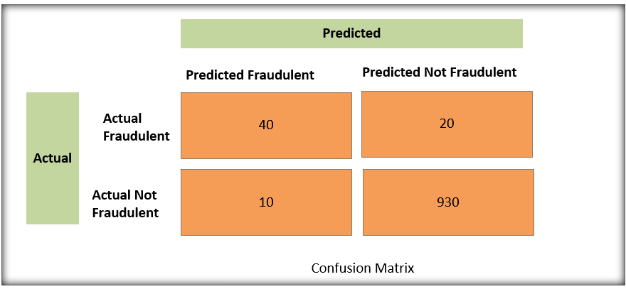
Interpreting the Matrix:
- 40 True Positives: The model correctly identified 40 fraudulent transactions.
- 930 True Negatives: The model correctly identified 930 legitimate transactions.
- 10 False Positives: The model incorrectly flagged 10 legitimate transactions as fraudulent (false alarms!).
- 20 False Negatives: The model missed 20 fraudulent transactions, classifying them as legitimate (missed opportunities!).
This allows us to quickly calculate and get a quick overview of how the model performs. It lets us to understand the performance, and where it could be improved. The false negatives is usually what we should focus on, since its usually better to make a false-positive than a false negative in fraud cases.
By looking at these counts, we can dive deeper into the model’s performance and tailor our strategies to address the specific errors. For instance, if we see too many false positives, we might adjust the model to be less sensitive and reduce false alarms. If we are missing many frauds, our metric should be Recall or F1 and then we need to focus on improving that metric.
For Regression Problems (predicting continuous values):
Imagine predicting customer lifetime value (CLTV).
- Mean Squared Error (MSE): Average squared difference between predicted and actual CLTV.
- Formula: MSE = (1/N) * Σ (y_i – ŷ_i)^2
- Considerations: Sensitive to outliers, which can disproportionately inflate the error.
- Root Mean Squared Error (RMSE): The square root of MSE, expressed in the same units as CLTV.
- Formula: RMSE = √(MSE)
- Interpretation: Represents the average magnitude of the prediction errors.
- Mean Absolute Error (MAE): Average absolute difference between predicted and actual CLTV.
- Formula: MAE = (1/N) * Σ |y_i – ŷ_i|
- Considerations: More robust to outliers than MSE/RMSE.
- R-squared (Coefficient of Determination): Proportion of variance in CLTV explained by the model.
- Formula: R-squared = 1 – (SSres / SStot)
- Interpretation: Ranges from 0 to 1. A value of 1 indicates the model perfectly explains the variation in CLTV, while 0 indicates it explains none of it.
2. Data Preparation: The Foundation of Reliable Evaluation
Your evaluation is only as good as the data you use. Proper data preparation is essential.
- Train/Validation/Test Split:
- Training Set: Used to train the model.
- Validation Set: Used to tune hyperparameters and prevent overfitting during training.
- Test Set: Used for a final, unbiased assessment of the model’s performance on unseen data.
- Cross-Validation: A technique for robustly estimating model performance by partitioning the data into multiple folds and iteratively training and evaluating the model on different combinations of folds.
- Addressing Imbalanced Data: Techniques like oversampling, undersampling, or cost-sensitive learning can help mitigate bias in models trained on datasets with uneven class distributions.
3. The Evaluation Process: Rigorous Experimentation
With goals defined, metrics chosen, and data prepared, it’s time to evaluate your model.
- Establish a Baseline: Compare your model’s performance against a simple rule-based approach, a random guess, or an existing system.
- Meticulous Tracking: Record all experimental details, including model architectures, hyperparameters, training data, and performance metrics.
- Focus on Generalization: Avoid overfitting to the training data. Regularly monitor validation set performance.
- Segmented Analysis: Evaluate performance across different demographic groups or data segments to identify potential biases.
- Error Analysis: Scrutinize individual errors made by the model to uncover patterns and areas for improvement.
4. Adversarial Robustness: A Modern Consideration
In today’s world, it’s not enough for your model to perform well on standard datasets. You also need to consider its resilience to adversarial attacks.
- What are Adversarial Attacks? Subtle perturbations to input data designed to fool the model into making incorrect predictions.
- Why are they Important? Malicious actors can exploit vulnerabilities in your model for nefarious purposes.
- How to Evaluate Robustness? Generate adversarial examples and assess the model’s accuracy on this perturbed data. This can be achieved using libraries like Cleverhans or Foolbox. Measuring the minimum perturbation needed to cause a misclassification (e.g., L-infinity norm) is also a common approach.
- Example: In an image recognition system, an attacker could add a nearly imperceptible pattern to an image of a stop sign, causing the model to classify it as a speed limit sign.
5. Interpretation and Communication: Translating Numbers into Insights
Performance metrics are valuable, but they need to be interpreted within the broader context of your problem.
- Context Matters: A high accuracy score might be meaningless if the problem is trivial.
- Visualization: Use charts and graphs to illustrate your findings.
- Trade-off Analysis: Acknowledge the trade-offs between different metrics.
- Stakeholder Communication: Clearly articulate your model’s strengths, limitations, and potential impact to non-technical audiences.
Conclusion
Measuring ML model performance is an ongoing process that requires careful planning, meticulous execution, and thoughtful interpretation. By selecting the right metrics, preparing your data rigorously, and considering modern challenges like adversarial robustness, you can unlock the full potential of your models and create solutions that deliver genuine value. Happy modeling!