
Do you need to predict future trends based on historical data? Want an easy-to-use tool that handles data upload, date frequencies, and generates interactive charts? Look no further! This blog post introduces a forecasting app built with Streamlit, Python, and a dash of data science magic.
Here is the link of application to try with your data: Forecasting APP
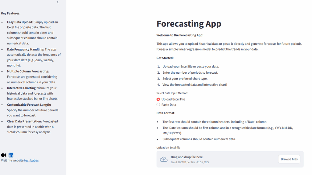
What is this app all about?
This app empowers you to easily forecast future values based on time-series data. Whether you’re tracking sales, inventory, website traffic, or anything else that changes over time, this app can help you peek into the future. It’s perfect for small businesses, analysts, or anyone who wants to make data-driven decisions.
Key Features:
- Effortless Data Import: Upload your data as an Excel file (XLSX or XLS) or simply paste it directly.
- Intelligent Date Handling: The app automatically recognizes the frequency of your date data (daily, weekly, monthly, etc.).
- Multi-Column Forecasting: It forecasts all numerical columns in your dataset, providing a comprehensive view of future trends.
- Interactive Visualizations: Choose between line and stacked bar charts to visualize historical data and forecasts.
- Customizable Prediction Length: Set the number of future periods you want to predict.
- Clear Data Presentation: The app presents forecasted data in a user-friendly table format, including a ‘Total’ column for easy analysis.
How it Works: A Behind-the-Scenes Look
The app leverages the power of Python and several key libraries:
- Streamlit: The framework for building the interactive web application.
- Pandas: Used for data manipulation and analysis, including reading and processing the uploaded data.
- Scikit-learn (sklearn): Provides the LinearRegression model for forecasting. The current implementation uses a simple linear regression model. For more complex forecasting scenarios, consider exploring more advanced time series models (e.g., ARIMA, Prophet). Future versions of the app could incorporate model selection.
- Matplotlib: Used for creating the interactive charts.
Example Usage:
- Prepare your data: Create an Excel file (or paste data) with a “Date” column (first column) and other numeric columns. For example:
Date,Sales,Marketing-Spend 2023-01-01,100,502023-01-08,120,602023-01-15,110,552023-01-22,130,65- Upload or paste: Upload the Excel file or paste the data into the app.
- Configure: Set the number of periods to forecast (e.g., 4 weeks) and select your preferred chart type (bar or line).
- Analyze: The app will display the forecasted data in a table and generate an interactive chart.
Here’s a breakdown of the core functions:
- preprocess_data(df, date_column=’Date’):
- Validates the input DataFrame.
- Ensures the specified date column (Date by default) is the first column and exists.
- Converts the date column to the correct datetime format.
- Sets the date column as the DataFrame’s index.
- Verifies that all other columns contain numeric data.
- Handles potential errors gracefully with informative error messages displayed in the Streamlit app.
def preprocess_data(df, date_column='Date'):
    """
    Preprocesses the data, handling different date frequencies.

    Args:
        df: Pandas DataFrame with 'Date' column and numerical columns.
        date_column: Name of the date column (default: 'Date').

    Returns:
        DataFrame with 'Date' as index and correctly formatted.  Returns None if
        the input DataFrame is invalid or an error occurs during preprocessing.
    """
    try:
        # Ensure 'Date' column exists and is the first column
        if date_column not in df.columns or df.columns[0] != date_column:
            st.error(f"Error: '{date_column}' column not found as the first column in the DataFrame.")
            return None

        # Convert 'Date' column to datetime
        df[date_column] = pd.to_datetime(df[date_column])

        # Set 'Date' as index
        df = df.set_index(date_column)

        # Ensure all remaining columns are numeric
        numeric_cols = df.select_dtypes(include=np.number).columns
        non_numeric_cols = df.columns.difference(numeric_cols)
        if len(non_numeric_cols) > 0:
            st.error(f"Error: Non-numeric columns found: {', '.join(non_numeric_cols)}. Please ensure all columns other than '{date_column}' contain only numbers.")
            return None

        if len(numeric_cols) == 0:
            st.error("Error: No numeric columns found in the DataFrame.")
            return None


        return df  # DataFrame with date index and numeric columns
    except Exception as e:
        st.error(f"An error occurred during data preprocessing: {e}")
return None- forecast(df, n_periods, model_type=’linear_regression’):
- Creates a time_index column representing the time sequence.
- Trains a LinearRegression model using the time_index as the predictor and other numeric columns as the target variables.
- Generates future dates based on the inferred frequency of the historical data.
- Predicts future values using the trained model.
- Calculates and adds a ‘Total’ column that sums up all other column values.
- Handles errors during the process and returns None if any arise.
def forecast(df, n_periods, model_type='linear_regression'):
    """
    Trains a linear regression model on the historical data and forecasts future values.

    Args:
        df: Pandas DataFrame with date index and numerical columns.
        n_periods: Number of periods to forecast.
        model_type: Type of model to use (default: 'linear_regression').  Currently only supports linear regression.

    Returns:
        DataFrame with forecasted values. Returns None if training fails.
    """
    try:
        # Create a sequence of numbers for time
        df['time_index'] = range(len(df))

        # Prepare data for training.  Use all numeric columns as features.
        X = df[['time_index']]  # Only use time_index as predictor
        y = df.drop('time_index', axis=1) # Target is all numeric columns

        # Train the model (no need for train/test split as we use all data for training for forecasting)
        model = LinearRegression()
        model.fit(X, y)

        # Generate future time index
        future_index = np.array(range(len(df), len(df) + n_periods)).reshape(-1, 1)

        # Make predictions
        forecast_values = model.predict(future_index)
        forecast_df = pd.DataFrame(forecast_values, columns=y.columns)

        # Create future date index
        last_date = df.index[-1]
        date_frequency = pd.infer_freq(df.index)  # Infer date frequency.  This is crucial.

        if date_frequency is None:
            st.error("Error: Could not infer date frequency.  Please ensure your date data has a consistent frequency (e.g., daily, weekly, monthly).")
            return None

        future_dates = pd.date_range(start=last_date, periods=n_periods + 1, freq=date_frequency)[1:] #Skip the first date as its already present
        forecast_df.index = future_dates

        # Add the total count column
        forecast_df['Total'] = forecast_df.sum(axis=1)


        return forecast_df

    except Exception as e:
        st.error(f"An error occurred during forecasting: {e}")
return None- plot_forecast(history_df, forecast_df, chart_type=’bar’):
- Creates a Matplotlib plot to visualize the historical and forecasted data.
- Offers a choice between a line chart and a stacked bar chart.
- For bar charts, it displays the values inside each segment of the bar and the total value on top, enhancing readability.
- Formats the x-axis to clearly display dates.
- Includes labels, titles, and a grid for better presentation.
def plot_forecast(history_df, forecast_df, chart_type='bar'):
    """
    Plots historical and forecast data using matplotlib.

    Args:
        history_df: Pandas DataFrame of historical data.
        forecast_df: Pandas DataFrame of forecasted data.
        chart_type: Type of chart to plot ('line' or 'bar').
    """

    try:
        plt.figure(figsize=(12, 6))
        if chart_type == 'line':
            for column in history_df.columns:
                plt.plot(history_df.index, history_df[column], label=f'Historical - {column}')
                plt.plot(forecast_df.index, forecast_df[column], label=f'Forecast - {column}')
        elif chart_type == 'bar':
            # Stacked bar chart
            x_hist = np.arange(len(history_df.index))
            x_forecast = np.arange(len(forecast_df.index)) + len(history_df.index)

            # Define a list of colors.  Make sure it has enough colors for all columns.
            colors = plt.cm.get_cmap('tab20').colors # or any other colormap

            # Calculate totals for historical and forecast data
            historical_totals = history_df.sum(axis=1)
            forecast_totals = forecast_df.drop('Total', axis=1).sum(axis=1) # Exclude 'Total' col, it is already sum of all columns


            # Plot historical data
            bottom = np.zeros(len(history_df.index))
            for i, column in enumerate(history_df.columns):
                color = colors[i % len(colors)]  # Cycle through colors if needed
                bars = plt.bar(x_hist, history_df[column], bottom=bottom, label=f'Historical - {column}', color=color)
                bottom += history_df[column]

                # Add numbers inside bars
                for bar in bars:
                    yval = bar.get_height()
                    if yval > 0.1: # Only show text if the segment is large enough
                        plt.text(bar.get_x() + bar.get_width()/2, bar.get_y() + yval/2, int(round(yval, 0)), ha='center', va='center', color='white', fontsize=8) #Center vertically too

            # Plot forecast data
            bottom_forecast = np.zeros(len(forecast_df.index))  # Use separate 'bottom' for forecast
            for i, column in enumerate(forecast_df.columns):
                if column != 'Total': # Don't include 'Total' in stacked bars.
                    color = colors[i % len(colors)]  # Cycle through colors if needed
                    bars = plt.bar(x_forecast, forecast_df[column], bottom=bottom_forecast, label=f'Forecast - {column}', color=color)
                    bottom_forecast += forecast_df[column]

                    # Add numbers inside bars
                    for bar in bars:
                        yval = bar.get_height()
                        if yval > 0.1: # Only show text if the segment is large enough
                            plt.text(bar.get_x() + bar.get_width()/2, bar.get_y() + yval/2, int(round(yval, 0)), ha='center', va='center', color='white', fontsize=8) #Center vertically too


            # Add total labels on top of the historical bars
            for i, total in enumerate(historical_totals):
                plt.text(x_hist[i], np.sum(history_df.iloc[i].values), int(round(total, 0)), ha='center', va='bottom', color='black', fontsize=10)

            # Add total labels on top of the forecast bars
            for i, total in enumerate(forecast_totals):
                plt.text(x_forecast[i], np.sum(forecast_df.drop('Total', axis=1).iloc[i].values), int(round(total, 0)), ha='center', va='bottom', color='black', fontsize=10)


            # Format x-axis to show only the date
            plt.gca().xaxis.set_major_formatter(mdates.DateFormatter('%Y-%m-%d'))
            plt.gca().xaxis.set_major_locator(mdates.AutoDateLocator())

            plt.xticks(np.concatenate([x_hist, x_forecast]), list(history_df.index.strftime('%Y-%m-%d')) + list(forecast_df.index.strftime('%Y-%m-%d')), rotation=45) #Label with dates


        plt.xlabel('Date')
        plt.ylabel('Value')
        plt.title('Historical and Forecast Data')
        plt.legend()
        plt.grid(True)
        plt.tight_layout() #Prevent labels from overlapping
        st.pyplot(plt)

    except Exception as e:
        st.error(f"An error occurred during plotting: {e}")
4. main()
Now write the main() function to call the above methods. This function orchestrates the entire Streamlit application:
- Title and Sidebar: Sets the app’s title and creates a sidebar for data input options and user information.
- Data Input: Provide options for uploading data from an Excel file or pasting data directly. Includes instructions on data format.
- User Input: Prompt the user to enter the number of periods to forecast and select the desired chart type.
- Function Calls: Calls the preprocess_data(), forecast(), and plot_forecast() functions to process the data, train the model, generate forecasts, and visualize the results.
- Data Display: Display the forecasted data in a Pandas DataFrame.
- Error Handling: Implement comprehensive error handling to gracefully manage potential issues at each stage of the process.
Conclusion:
This Streamlit forecasting app offers a user-friendly way to generate forecasts using a linear regression model. Its strength lies in its ease of use, data preprocessing capabilities, and interactive visualizations. While the model itself is relatively simple, the app provides a solid foundation for exploring time series data and generating basic forecasts. By incorporating more advanced models and feature engineering techniques, you can further enhance the app’s accuracy and predictive power.
For more AI blogs visit my medium blog page: Anil Tiwari – Medium
Follow me on LinkedIn: https://www.linkedin.com/in/aniltiwari/
Awesome
Awesome
Good
Good
Awesome
Very good
Very good
Very good
Good
Awesome
Awesome
Very good